Capital Equipment Value Models

Table of Contents

• Introduction
• Simple Value Model
• Adjacent-Effects Value Model
• Defect-Processing Value Model
• Time-to-Profit Value Model
• Capital-Life Value Model
• What Price Should You Use?

Introduction

It is time to turn the concept of value into some hard numbers. First, recall these three important value-based strategy principles:

1. The customer defines value.
2. Value is relative to alternatives.
3. Value is a financial expression.

You will use these principles to develop value models that show the financial outcome of your customer’s buying decision and reveal your value proposition.

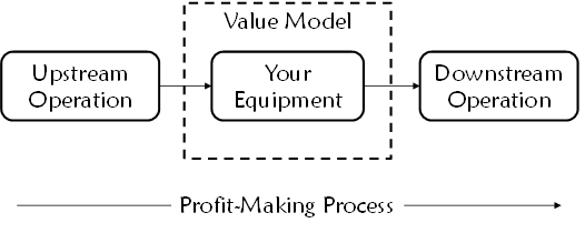
These value models take the form of financial statements that compare the financial outcome of buying your equipment versus the next best alternative. The difference is your value proposition. See Figure 21.

You can model the economics of all capital equipment buying decisions using comparative financials. However, the structure of your model will depend on the role your equipment plays in your customer’s profit-making process.

Consider these questions:

• Is the buying decision limited to the economics of the operation that your equipment performs?
• Does the decision to buy your equipment include consideration for how it affects the economics of other equipment or operations?
• Is the equipment buyer purchasing for production or for research and development?
• Is your equipment employed to resolve production failures?
• Does the buying decision for your equipment include consideration for some future revenue source with different process requirements?

Your answers will help you determine which of the following value models or combination of models is the most appropriate starting point for your situation.

Simple Value Model

In the simple value model, the buying decision considers the time from the moment the workpiece enters your equipment to the moment it exits. It applies if your equipment operates in series with the customer’s primary profit-making process and only the process your equipment performs drives the economics of the purchasing decision. With the simple value model, you only need to consider the buying decision drivers related to the operation of your equipment. See Figure 22.

Let us again turn to Mr. Melty. In this scenario, you have learned that your customer needs one system and defines value as the cost to manufacture one kilogram of multicrystalline silicon. Your market intelligence has also revealed the data in Table 11.

Buying Decision Driver	Mr. Melty	Competitor
Charge size	650 kg	700 kg
Process time	<65 hrs	<75 hrs
Yield	>75%	>65%
Price	$655K	$600K

With this data, you can develop a value model to calculate your equipment’s value compared to the competition. See Figure 23.

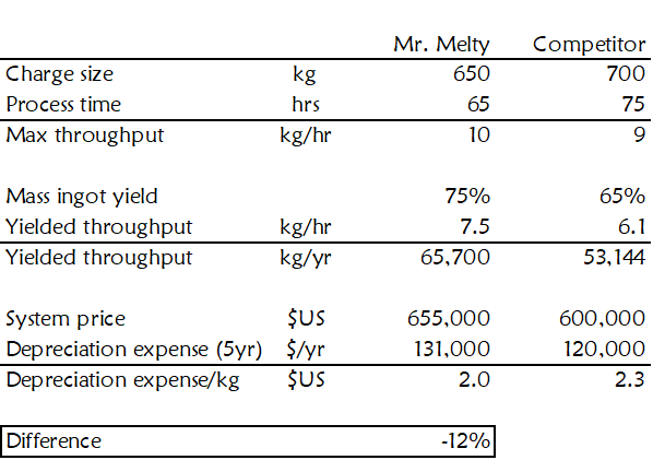
You will notice the following from the example in Figure 23:

• The value model limits the analysis to the buying decision drivers.
• Buying decision drivers, throughput, and yield define ingot growth furnace output.
• Equipment price is the only cost where material differences exist.
• You must convert system prices to an annual depreciation expense to match the output units of kg/year.
• When Mr. Melty’s price is $655,000 and the competitor’s price is $600,000, the buyer can expect to save 12% in depreciation expense/kg by buying Mr. Melty.

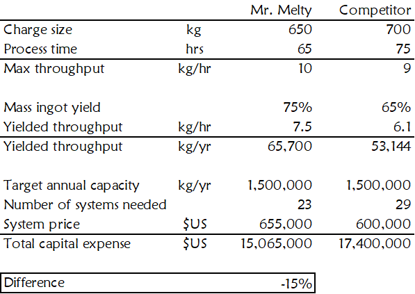
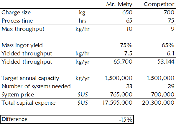
Another simple value model scenario occurs when the buyer is buying to satisfy a specific capacity, as is often the case for production equipment. See Figure 24.

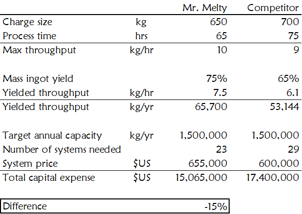
Note that the percentage difference in value in the fixed-machine-number and fixed-capacity value models may be different. This is due to rounding up to the number of whole machines needed in the fixed-capacity financials.

Operating costs can also be buying decision drivers in certain circumstances, such as:

• Competing systems have the same or similar capital depreciation expense per unit output but have meaningful differences in operating costs.
• Competing systems have meaningful capital depreciation expense per unit output differences and operating cost differences of a similar scale.

See Figure 25 for an example.

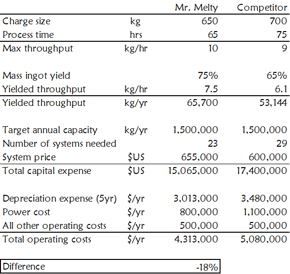
You will notice the following from the example in Figure 25:

• Since companies express operating costs over time, you will need to express equipment price as an annual depreciation expense to keep units consistent.
• Mr. Melty and its competitor have meaningful capital depreciation expense differences and operating cost differences of a similar scale.
• Power cost is the element of the operating costs that contributes to the buying decision.
• The model includes all other costs since excluding them would exaggerate the financial outcome difference between the buying choices.

Adjacent-Effects Value Model

When the purchasing decision for your type of equipment also considers the economics of adjacent equipment or operations, the adjacent-effects value model applies. This model is often appropriate when any of the following materially affects your customer’s buying decision:

• The economics of upstream operations
• The economics of downstream operations
• The value of your customer’s product

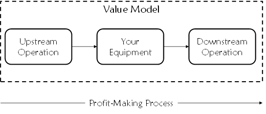
For example, if your equipment affects the economics of the operations immediately up and downstream of your equipment, your value model would take the form shown in Figure 26.

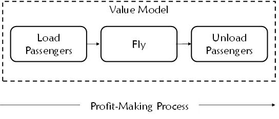
Consider an airline that is evaluating the purchase of several jumbo passenger jets. The airline’s choices are the Airbus A380 and the Boeing B747. One unique feature of the A380 is that it has two passenger decks that run the full length of the plane. The two full-length decks are the source of its capacity advantage over the B747, which has a full-length main deck but only a small second deck in the front.

However, to load and unload passengers from the A380’s two decks in parallel, its buyers need to build and install special two-story jet bridges. Not so for the B747. It only loads and unloads passengers from the main deck. So, its buyers can use their existing single-story jet bridges. In this example, the purchasing decision for jumbo jets considers the economics of flying the jet plus loading and unloading passengers. Therefore, the adjacent-effects value model applies. See Figure 27.

An extreme case of an adjacent-effects value model is when the economics of the buyer’s entire profit-making process drives the buying decision for a single piece of equipment. Here, the value model will include all equipment and operations. This extreme case usually appears when the revenue the equipment buyer can get for each unit of its product, or the yield of its entire operation drives the buying decision.

For example, solar cell manufacturers are in the business of selling power. The amount of power produced by a solar cell determines its price. A cell that produces twelve watts of power might sell for $12.00, while a cell that produces ten watts of power might sell for $10.00.

Turning a bare silicon wafer into a solar cell requires dozens of equipment types. Suppose you sell one of these equipment types, and its primary buying criteria include the amount of power, and therefore revenue that each solar cell produces. The value model for your piece of equipment must consider the entire profit-making process because it will include the revenue-per-unit factor. It takes an entire factory to produce revenue. To express the economic benefit of your equipment, you need a value model like the one shown in Figure 28.

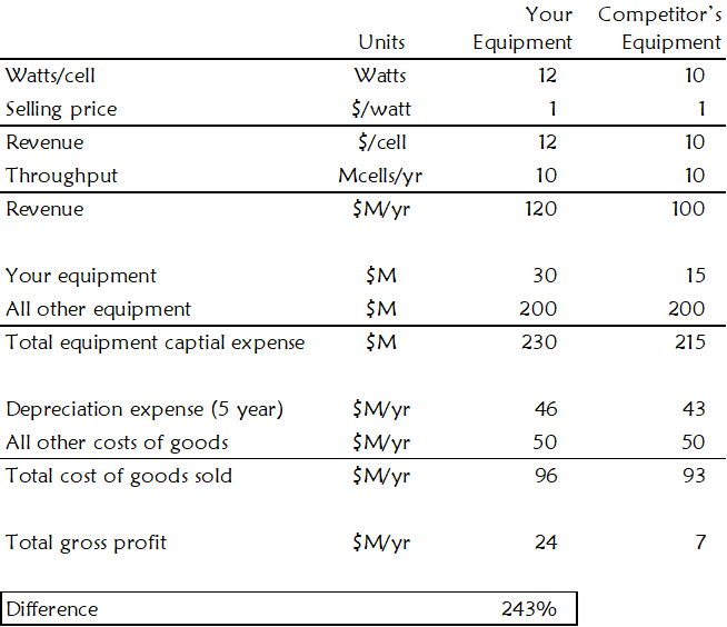
In this example, your value proposition is that spending $30M on your equipment will produce 243% more annual gross profit than spending $15M on your competitor’s equipment.

Notice the incredible pricing leverage you have in this example. This leverage occurs when the financial outcome of the entire profit-making process drives the buying decision, and your equipment is a small fraction of the total cost. In most cases, the broader your adjacent-effects scope, the more value-based pricing leverage you will have.

However, the difficulty of substantiating your value during a sales process is also directly proportional to the adjacent effects scope. In this example, to substantiate your value, you would need to understand the economics of the entire profit-making process, not just the economics of your equipment, and substantiate that your equipment deserves credit for the added profit.

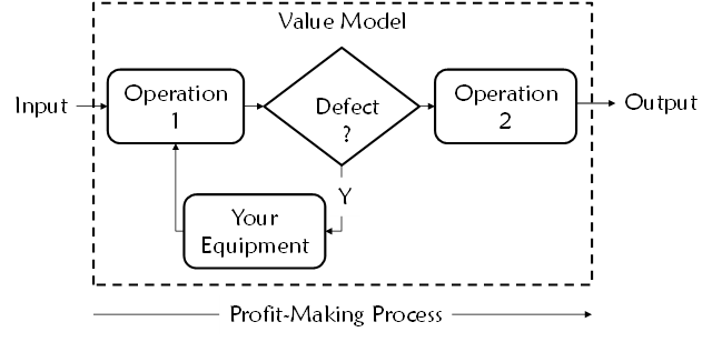
Defect-Processing Value Model

Defect-processing equipment often lives in failure analysis labs or quality control departments. It typically receives a workpiece anytime that a defect takes down the profit-making process or causes it to run inefficiently. Differences in the time it takes for defect-processing equipment to resolve a defect affect throughput, uptime, yield, or costs for part or all the profit-making process. See Figure 29.

Buyers of defect-processing equipment are usually more concerned with the equipment’s cycle time than they are with throughput. Throughput and cycle time are related, but not the same. Cycle time is the time that your equipment takes to process one unit. Throughput is the total number of units your equipment can process over a specified time. Faster defect-processing cycle times reduce downtime in the profit-making process.

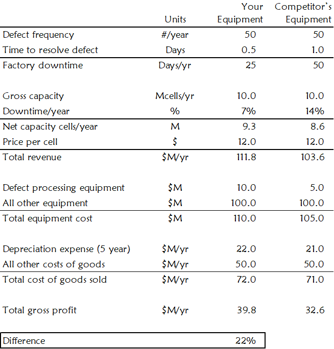
For example, suppose your equipment processes a certain catastrophic defect in the production of solar cells. When this defect occurs, the solar cell manufacturer must stop the production line and resolve it.

Here, the defect-processing equipment affects the solar cell manufacturer’s profit in two ways. First, a defect results in downtime for the factory. The defect resolution cycle time determines how long the factory will be down for each defect and, therefore, affects the overall throughput of the factory. Second, the defect-processing equipment is not free. It will burden the buyer with depreciation expense and operating costs. See Figure 30.

Time-to-Profit Value Model

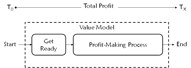
Sometimes buyers intend to use your equipment to get ready to make a profit. Research and development equipment, for example, performs this function. The value of your equipment, in this case, relates to how quickly it helps the customer get to the profit-making process.

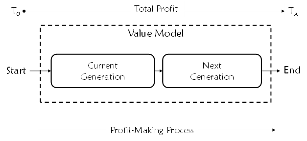
The value model for this scenario considers the total profit from the time the get-ready process starts to some relevant time after profit making begins. See Figure 31.

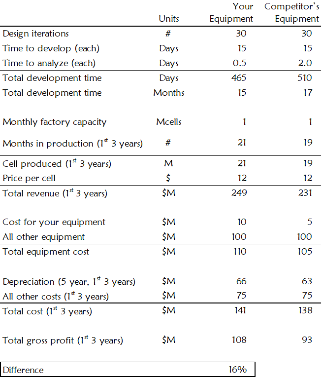
To illustrate, let us try another example. Suppose a solar power company is developing its next-generation solar cell. During that development, the company will need to analyze the results of many design iterations before the solar cell design is ready for production.

You have developed a system that can analyze design iterations in a quarter of the time it takes your nearest competitor. During its demonstration, your customer confirmed that your equipment will shave two months off their next-generation cell development time.

But you want to figure out how much getting to production two months earlier is worth to your customer. Then, once you understand that, how to price your equipment to reflect its value. Your value model might look like the one in Figure 32.

Capital-Life Value Model

When your customer’s buying decision considers the period that your equipment can produce revenue, the capital-life value model may apply. See Figure 33.

There are two common situations where this model applies. The first is when the buying decision considers the need to replace the equipment because of an irreparable failure. The second is when the buying decision considers the equipment capability over multiple generations of the customer’s product.

For example, in semiconductor device manufacturing, each device generation requires new equipment that can process smaller features and new materials. When the buying decision considers the equipment’s ability to process future product generations, the capital-life value model is appropriate.

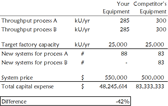
To illustrate, suppose your equipment is five percent slower than your competitor and costs more per system. However, only your equipment can produce process-A products and next-generation process-B products.

If your customer chooses your competitor, he will need to buy a new set of equipment when he switches his factory over to process B. Despite being slower and more expensive, you can still save the customer a lot of money. See Figure 34.

What Price Should You Use?

For internal value analysis, use expected final prices for you and your competitor. When the value model is customer facing, the price you show depends on where you are in the sales process. Early in the sales process, use something akin to a list price. Deep into final negotiations, use something near the expected purchase price. See Table 12.

Use Case	What Price to Use
Product Strategy	Expected purchase price
Market Requirements Document	Expected purchase price
Standard Sales Kit	List price
Sales Cycle	Start at list, then migrate to the expected purchase price as discovery and negotiations proceed

Let us return to the Mr. Melty example. Imagine your task is to communicate price to your prospect early in the sales process. Here, you need to establish a list price.

Real estate agents do this when they list a house for sale. The real estate agent conducts a market assessment of your house’s value compared to other houses on the market. Then the agent recommends a list price that positions your house favorably among the list prices of other houses on the market.

Your task is the same but with one significant disadvantage compared with house sellers. You cannot log in to a multiple listing website to see other equipment makers’ list prices. However, you can use your competitor’s expected pricing to derive a proxy for their list price. To go from the expected purchase price to a list price in your value model, follow these three steps:

1. Use your value model to determine your value proposition at expected purchase prices for you and your competitor.
2. Select a list price for your equipment that is far enough from the expected purchase price to allow for negotiations.
3. Calculate a “list” price for your competitor’s equipment that when compared to your list price produces the same value proposition in your value model as when you used expected purchase prices.

For value models showing equivalent Mr. Melty value propositions using expected and list prices, see Figures 35 and 36.